Model Optimization Techniques
Performance optimization methods for LLMs and diffusion models using NVIDIA Model Optimizer
NVIDIA/Model-Optimizer📊 What is MMLU?
Massive Multitask Language Understanding (MMLU) is a benchmark designed to evaluate language models across a diverse range of subjects and tasks. Created by researchers at UC Berkeley, it has become the standard metric for measuring the impact of optimization techniques on model quality.
57 Subjects
Covers mathematics, philosophy, law, medicine, history, computer science, and more — testing broad knowledge.
~16,000 Questions
Multiple-choice format ranging from elementary to professional difficulty levels.
Why It Matters
MMLU loss measures how much reasoning ability is sacrificed for performance gains. Lower loss = better quality retention.
Reference: MMLU on Wikipedia | Original Paper (Hendrycks et al., 2020)
⚡ Overview
Model optimization reduces model size and increases inference speed while maintaining accuracy. The main techniques are:
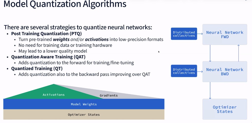
Post-Training Quantization (PTQ)
Reduce precision of weights and activations after training. Fast to apply, no retraining needed.
Up to 2.1x speedupQuantization-Aware Training (QAT)
Train the model knowing it will be quantized. Better accuracy at ultra-low precision (4-bit).
Better accuracySparsity
Prune weights to zero, reducing compute. Combine with fine-tuning for best results.
Up to 1.62x speedupAWQ (Activation-aware Weight Quantization)
Smart 4-bit quantization preserving important weights. Memory-efficient for large models.
4x memory reduction📖 Understanding Each Technique
FP8 Post-Training Quantization (FP8 PTQ)
FP8 (8-bit floating point) quantization converts model weights and activations from higher precision formats (FP16/BF16) to 8-bit floating point after the model has been fully trained. Unlike integer quantization, FP8 preserves the floating-point format's ability to represent a wide dynamic range through its exponent bits, making it particularly well-suited for transformer models where activation values can vary significantly across layers.
How FP8 Works: FP8 comes in two variants—E4M3 (4 exponent bits, 3 mantissa bits) for weights and E5M2 (5 exponent bits, 2 mantissa bits) for activations. The E4M3 format provides higher precision within a narrower range, ideal for relatively stable weight distributions. E5M2 trades precision for dynamic range, handling the wider variance in activation values. During inference, FP8 values are multiplied directly on Tensor Cores, with results accumulated in FP16/FP32 for numerical stability.
The Calibration Process: PTQ requires a calibration step using a small representative dataset (typically 128-512 samples). The model runs forward passes on this data while the quantizer collects statistics—minimum, maximum, and distribution of values for each tensor. From these statistics, per-tensor or per-channel scaling factors are computed to map the FP16 range to FP8. The choice of calibration algorithm (MinMax, Entropy, Percentile) affects the trade-off between clipping outliers and preserving precision for common values.
The key advantage of FP8 PTQ is its simplicity: you take a trained model, run calibration, and convert the weights. No retraining required. Modern GPUs like H100 and H200 have native FP8 Tensor Core support, enabling direct hardware acceleration. This makes FP8 the default recommendation for production LLM deployments on NVIDIA hardware—delivering up to 2.1x speedup with less than 1.5% accuracy degradation.
Reference: NVIDIA NeMo Quantization Guide | FP8 Formats for Deep Learning (Micikevicius et al., 2022)
INT4 AWQ (Activation-Aware Weight Quantization)
AWQ is a weight-only quantization method that compresses model weights to just 4 bits (INT4) while keeping activations in higher precision during computation. The "activation-aware" aspect is crucial: AWQ identifies which weight channels are most important by analyzing activation patterns, then protects these salient weights from aggressive quantization while compressing less critical weights more aggressively.
How AWQ Identifies Salient Weights: AWQ observes that not all weights contribute equally to model output. By running calibration data through the model, AWQ measures activation magnitudes for each channel. Weights connected to channels with large activations are "salient"—small errors in these weights get amplified by large activations, causing significant output degradation. AWQ computes a per-channel importance score: importance = mean(|activation|). The top 1% of channels by importance are identified as salient.
The Scaling Trick: Rather than keeping salient weights in higher precision (which would complicate hardware), AWQ uses a clever mathematical equivalence. For a linear layer Y = XW, multiplying weights by a scale s and dividing activations by the same scale gives identical results: Y = (X/s)(sW). AWQ scales up salient weight channels before quantization, effectively giving them more of the INT4 range's precision. During inference, the activation is scaled down to compensate. This keeps all weights in INT4 format while protecting important channels from quantization error.
Group Quantization: AWQ typically uses group-wise quantization, where weights are divided into groups of 128 consecutive values, each with its own scale factor. This provides finer granularity than per-tensor quantization, capturing local value distributions. The scale factors are stored alongside the 4-bit weights, adding ~3% memory overhead but significantly improving accuracy.
This approach achieves approximately 4x memory reduction compared to FP16, allowing you to fit larger models on fewer GPUs. The trade-off is throughput: INT4 AWQ can be slower than FP8 at higher batch sizes because it requires dequantization to FP16 before Tensor Core operations. Use INT4 AWQ when memory is your primary constraint—for example, serving a 70B model on a single GPU instead of two.
Reference: AWQ Paper (Lin et al., 2023)
W4A8 AWQ (4-bit Weights, 8-bit Activations)
W4A8 extends AWQ by also quantizing activations to 8 bits (INT8) during matrix multiplications, not just the weights. This enables the use of INT8 Tensor Cores for the actual computation, which can provide better throughput than weight-only INT4 quantization that requires dequantization to FP16 for each operation.
How W4A8 Computation Works: In pure weight-only INT4 (W4A16), the INT4 weights must be dequantized to FP16 on-the-fly before matrix multiplication, because FP16 activations cannot directly multiply with INT4. This dequantization overhead limits throughput. W4A8 solves this by quantizing activations to INT8 dynamically at runtime. The INT4 weights are pre-converted to INT8 (by unpacking and zero-point adjustment), enabling direct INT8×INT8 matrix multiplication on Tensor Cores with INT32 accumulation.
Dynamic vs Static Activation Quantization: Weights are quantized once (static), but activations must be quantized per-token at runtime (dynamic) since their values depend on input. W4A8 computes per-token or per-tensor activation scales on-the-fly: scale = max(|activation|) / 127. This adds a small overhead but enables INT8 Tensor Core utilization. The per-token quantization is critical for LLMs where different sequence positions can have vastly different activation magnitudes.
W4A8 represents a balanced approach: you get most of the memory savings from 4-bit weights (enabling larger models) while gaining computational efficiency from INT8 Tensor Core operations. The accuracy impact is slightly higher than FP8 due to the additional activation quantization, but W4A8 often outperforms pure INT4 AWQ in throughput, especially at larger batch sizes where Tensor Core utilization dominates. It's ideal when you need both memory efficiency and high throughput.
Quantization-Aware Training (QAT)
QAT fundamentally differs from PTQ by incorporating quantization simulation into the training process itself. During forward passes, weights and activations are quantized to the target precision; during backward passes, gradients flow through using the "straight-through estimator" to enable learning. This allows the model to adapt its weights to compensate for quantization error during training.
The Fake Quantization Mechanism: QAT inserts "fake quantization" nodes into the computational graph. During the forward pass, these nodes simulate quantization: q(x) = round(x/scale) × scale. The output is still in floating-point but has been rounded to values representable in the target precision. This lets the model "experience" quantization error during training. The loss function sees the quantized outputs, so gradients naturally push the model toward weights that are robust to rounding.
Straight-Through Estimator (STE): The rounding operation has zero gradient almost everywhere (it's a step function), which would block backpropagation. STE solves this by pretending the gradient of rounding is 1: during backward pass, gradients flow through the fake quantization node unchanged, as if it were an identity function. Mathematically: ∂q(x)/∂x ≈ 1. This approximation works surprisingly well in practice—the model learns to place weights where rounding causes minimal damage.
QAT Training Process: Typically, QAT starts from a pre-trained FP16 model and fine-tunes for 5-10% of the original training steps. The quantization parameters (scales, zero-points) are learned jointly with the weights—either frozen after a warmup period or updated throughout. For LLMs, QAT often uses a small subset of the original training data or a task-specific dataset. The compute cost is modest (hours to days, not weeks), making QAT practical even for large models.
The benefit becomes dramatic at ultra-low precisions. When quantizing to INT4 weights with INT8 activations, PTQ can cause validation loss to explode (e.g., 1.036 → 3.321), while QAT maintains much better accuracy (1.036 → 1.294). QAT is essential for accuracy-critical applications targeting aggressive quantization, and it's particularly important for deploying 4-bit models on NVIDIA Blackwell architecture which has native 4-bit Tensor Core support.
Reference: QAT Paper (Jacob et al., 2017) | Integer Quantization for Deep Learning (Wu et al., 2020)
Sparsity (Weight Pruning)
Sparsity reduces computation by setting a portion of model weights to exactly zero. NVIDIA's sparse Tensor Cores support 2:4 structured sparsity, where exactly 2 out of every 4 consecutive weights are zero. This structured pattern allows hardware to skip computations for zero weights, achieving up to 2x theoretical speedup while storing only the non-zero weights plus a small index overhead.
2:4 Structured Sparsity Explained: In 2:4 sparsity, weights are processed in groups of 4. Within each group, exactly 2 weights are pruned to zero based on magnitude—the smallest two are removed. The remaining 2 non-zero weights are stored compactly, along with a 2-bit index indicating their positions. For example, weights [0.5, -0.1, 0.8, 0.2] become [0.5, 0, 0.8, 0] stored as [0.5, 0.8] with index [0, 2]. This achieves 50% weight reduction with predictable memory layout.
Hardware Acceleration: NVIDIA Ampere and later GPUs have Sparse Tensor Cores that exploit this pattern. During matrix multiplication, the hardware reads only the non-zero weights and uses the index to correctly align them with input activations. Since exactly half the weights are zero, the Tensor Core performs half the multiply-accumulate operations, achieving up to 2x speedup for compute-bound operations. The actual speedup (1.3-1.6x in practice) is lower due to memory bandwidth and other overheads.
Pruning Methods: Several algorithms exist for inducing 2:4 sparsity. Magnitude pruning simply zeros the smallest weights in each group—fast but often hurts accuracy. SparseGPT uses second-order information (Hessian) to choose which weights to prune while compensating remaining weights to minimize output change—better accuracy but slower. Wanda (Weights and Activations) considers both weight magnitude and activation magnitude, similar to AWQ's insight. All methods benefit significantly from post-pruning fine-tuning.
The critical insight from benchmarks is that sparsity without fine-tuning causes severe accuracy degradation (validation loss jumping from 0.721 to 2.724 in Llama 2-70B). However, combining sparsity with fine-tuning on target data recovers most accuracy (0.721 → 1.01) while maintaining significant speedups. Sparsity can be combined with quantization (e.g., FP8 + sparsity) for compound gains—the MLPerf Inference v4.0 submission used this combination to achieve record performance.
Reference: NVIDIA Sparsity Guide | SparseGPT (Frantar & Alistarh, 2023) | Wanda (Sun et al., 2023)
🔢 Post-Training Quantization for LLMs
Tested on H200 with TensorRT-LLM v0.15. Input: 2048 tokens, Output: 128 tokens.
Llama 3.1-8B Performance
| Batch Size | BF16 (baseline) | FP8 | INT4 AWQ | W4A8 AWQ |
|---|---|---|---|---|
| 1 | 173.8 tok/s | 245 tok/s (1.41x) | 231.8 tok/s (1.33x) | 239.7 tok/s (1.38x) |
| 8 | 803.1 tok/s | 1,051 tok/s (1.31x) | 599.7 tok/s (0.75x) | 801.7 tok/s (1.00x) |
| 64 | 1,679.7 tok/s | 2,191 tok/s (1.30x) | 1,392.8 tok/s (0.83x) | 1,930.9 tok/s (1.15x) |
Llama 3.1-70B Performance (GPU-count normalized)
| Batch Size | BF16 TP2 (baseline) | FP8 TP1 | INT4 AWQ TP1 | W4A8 AWQ TP1 |
|---|---|---|---|---|
| 1 | 45.8 tok/s | 43.5 tok/s (1.90x) | 44.1 tok/s (1.93x) | 46.3 tok/s (2.02x) |
| 8 | 182.6 tok/s | 182.1 tok/s (1.99x) | 94.0 tok/s (1.03x) | 140.0 tok/s (1.53x) |
| 64 | 401.5 tok/s | 420.6 tok/s (2.10x) | 176.7 tok/s (0.88x) | 345.4 tok/s (1.72x) |
Accuracy Impact (MMLU Loss vs BF16)
FP8
INT4 AWQ
W4A8 AWQ
🎨 PTQ for Stable Diffusion
Stable Diffusion XL 1.0 base, 1024×1024 resolution, 30 steps, batch size 1.
| GPU | INT8 Latency | FP8 Latency | INT8 Speedup | FP8 Speedup |
|---|---|---|---|---|
| RTX 6000 Ada | 2,479 ms | 2,441 ms | 1.43x | 1.45x |
| RTX 4090 | 2,058 ms | 2,161 ms | 1.20x | 1.14x |
| L40S | 2,339 ms | 2,168 ms | 1.25x | 1.35x |
🎯 Quantization-Aware Training (QAT)
QAT trains the model knowing it will be quantized, preserving accuracy at ultra-low precision. Enables 4-bit inference on NVIDIA Blackwell.
Llama 2-7B Validation Loss Comparison
| Method | Dataset | BF16 Baseline | PTQ | QAT |
|---|---|---|---|---|
| INT4 Weight, FP16 Act | samsum | 1.036 | 1.059 | 1.044 |
| INT4 Weight, INT8 Act | samsum | 1.036 | 3.321 | 1.294 |
| INT4 Weight, FP16 Act | dolly-15k | 1.151 | 1.305 | 1.172 |
| INT4 Weight, INT8 Act | dolly-15k | 1.151 | 2.313 | 1.640 |
🕸️ Sparsity
Pruning weights to zero reduces compute. Llama 2-70B on H100, FP8, TP=1. Part of MLPerf Inference v4.0.
Performance Gains
| Batch Size | Speedup vs Dense FP8 |
|---|---|
| 32 | 1.62x |
| 64 | 1.52x |
| 128 | 1.35x |
| 896 (MLPerf) | 1.30x |